Session Descriptor -
Learn the basics of Microsoft Excel 2013/2016 by learning ways to increase productivity and maximize visual representation and data analysis in the classroom. This training is designed for learners who are new to excel. Goals for this session are: learn basic terminology, data entry, data analysis, explanation of basic excel tools, and basic formatting tasks. Participants of this session will be able to create a basic spreadsheet and format it using the basic tools of excel.
Learn the basics of Microsoft Excel 2013/2016 by learning ways to increase productivity and maximize visual representation and data analysis in the classroom. This training is designed for learners who are new to excel. Goals for this session are: learn basic terminology, data entry, data analysis, explanation of basic excel tools, and basic formatting tasks. Participants of this session will be able to create a basic spreadsheet and format it using the basic tools of excel.
PLC Guiding Questions |
ISTE Standards |
Objectives |
Success Criteria |
|
ISTE Standards for Teachers: model and facilitate effective use of current and emerging digital tools to locate, analyze, evaluate, and use information resources to support research and learning Digital Citizenship Component: Privacy" "ISTE Standard for Students: collect data or identify relevant data sets, use digital tools to analyze them, and represent data in various ways to facilitate problem-solving and decision-making |
* Become familiar with terminology and tools. * Create a simple workbook * Add columns, rows, and pages * Explore the formatting options within a sheet or workbook * Create and explore formulas, sorting, and filtering * Add and edit borders within a worksheet * Create a simple chart |
* Participants can explain common basic excel vocabulary terms (spreadsheet, workbook, worksheet, cell, cell name, merge cell, border lines, grid- lines, sorting, filtering) * Participants can create a workbook. * Participants can add data to excel spreadsheet. * Participants can use basic text formatting in spreadsheet (i.e. color, font type, size, bold, italicize, underline). * Participants can add new and adjust column/row widths and heights. * Participants can adjust margins and page orientation (I.e. to fit data in printable document). * Participants can merge cells (i.e. to create headings for data table) * Participants can change the cell color. * Participants can add border lines. * Participants can use the sorting and filtering functions * Participants can use the AVERAGE formula to find the average of a column or row. * Participants can create a simple chart |
TEAM Rubric Instructional Plans, Use of Data
Standards CCSS Math, CCSS ELA, and Literacy/Science/Technology
Digital Citizenship Internet Safety, Privacy
Standards CCSS Math, CCSS ELA, and Literacy/Science/Technology
Digital Citizenship Internet Safety, Privacy
1. Terminology and Basic Navigation of the Excel Program
The Excel Worksheet
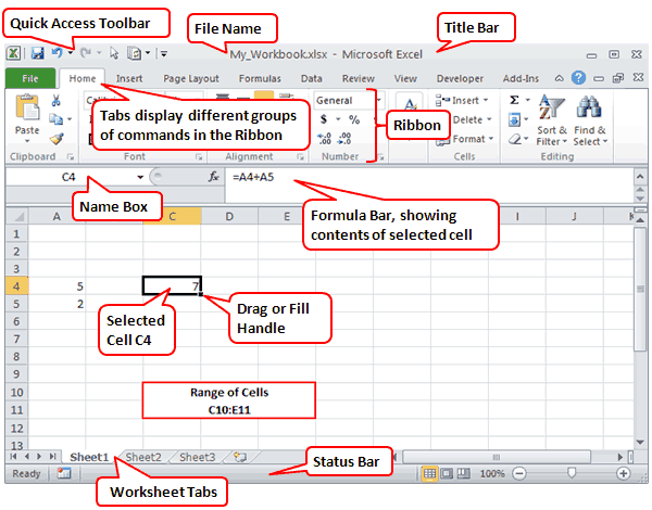
Terminology -
- Worksheet: a row and column matrix sheet on which you work.
- Spreadsheet: this type of computer application.
- Workbook: the book of pages that is the standard Excel document.
- Cell: the workbook is made up of cells. There is a cell at the intersection of each row and column. A cell can contain a value, a formula, or a text entry.
- Rows, Columns, and Sheets: The Excel worksheet contains 16,384 rows that extend down the worksheet, numbers 1 through 16384. The worksheet contains 256 columns that extend across the worksheet, lettered A through Z, AA through AZ, BA through BZ, and continuing IA through IZ. The Excel workbook can contain as many as 256 sheets, labeled Sheet 1 through Sheet 256. The initial number of sheets in a workbook, which can be changed by the user, is 16.
- Cell references: Cell references are the combination of column letter and row number. For example, the upper-left cell of a worksheet is A1.

|
Entering Data into a Spreadsheet1. In cell A1, type Keyboarding – 4th Period Grades
2. Type as follows:
4. Type in cells: B3 – 90; C3 – 75; and D3 - 95 5. Type in cells: B4 – 75; C4 – 80; and D4 – 75 6. Type in cells: B5 – 90; C5 – 85; and D5 – 85 7. Type in cell A6 – Average |
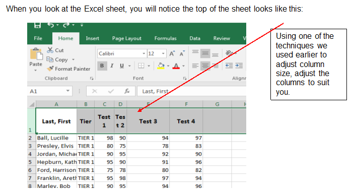
Changing Cell Size1. Point with your mouse between the A and B columns. When the cursor changes to a line crossed by a double- sided arrow, click and drag the column to the right. This will make the A column wider.
2. Point with your mouse between the B and C columns. When the cursor changes to a line crossed by a double- sided arrow, quickly double click the left mouse button. Notice that the column automatically adjusts to fit the text. 3. Adjust the width of all columns through E. |

|

|
Making Text Bold -1. Select cell A1 by clicking on the cell. Then, point to the B icon on the tool bar.
2. Bold the text in cells: A2; B2; C2; D2; E2; and A6. |
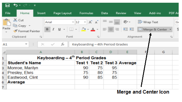
Merge and Center -Click in cell A1 and drag through cell E1 to select all cells. Release the left mouse button. With your mouse, click the Merge and Center icon on the toolbar. This will center your heading.
|

|
For Future Reference...Entering and Editing Data in Excel 2016 Video Tutorial
2. Formulas
A formula is an expression telling the computer what mathematical operation to perform upon a specific value. When referring to computer software, formulas are most often used in spreadsheet programs, such as Microsoft Excel. Using formulas in spreadsheets can allow you to quickly make calculations and get totals of multiple cells, rows, or columns in a spreadsheet.

|
Using a Formula
1. Click and highlight B3, C3, and D3
2. Click the dropdown menu icon next to the ∑ AutoSum and choose Average |
|
Copying Formula to Other Cells
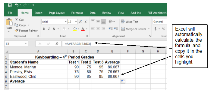
1. Point to the right bottom of cell E3 until you get the plus sign.
2. When you get the plus sign, click and hold down the left mouse button. 3. Drag through cell E5 4. Excel will automatically fill in averages for Cells E4 and E5. 5. Now use the same method as above to find the average for Test 1, this will be in Cell C6. Use the drag method to calculate the averages for Tests 2, Test 3, and Average. |

|
For Future Reference...10 Most Used Formulas in MS Excel
3. Adding Columns & Rows
|
|
In your new row A6 enter Woman, Wonder in B6 enter 95, C6 enter 100, D6 enter 90.
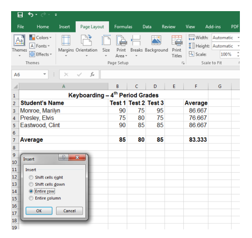
Now click on Column E and right click to choose "insert" from the pop up menu.
In E2 enter “Test 4” E3 enter 95, E4 enter 85, E5 enter 90, E6 enter 95
Now click on Column E and right click to choose "insert" from the pop up menu.
In E2 enter “Test 4” E3 enter 95, E4 enter 85, E5 enter 90, E6 enter 95

|
"How do we get the “Average” formula to extend to F6, and E7??"
|
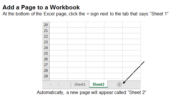
Naming a Page in a Workbook -
- Right click over top of tab that says “Sheet 1” and choose “rename” and call it “Keyboarding” then click OK.
- Right click over top of tab that says “Sheet 2” and choose “rename” and call it “Homeroom” click OK.
For Future Reference...Insert/Remove Columns, Rows, and Cells
4. Copying and Pasting
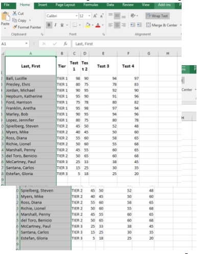
Now, let's copy and paste some data into this HOMEROOM sheet.
- Open the “Fake Homeroom” workbook. Select and highlight the data from the spreadsheet and use the CTRL + C keyboard shortcut to copy the data
- Go back to the “Inservice Excel Spreadsheet” workbook you’ve created and click on “Homeroom” tab. Right click in cell A1 and choose “paste”.
Ta-da!! You have just copied data from one Excel worksheet and pasted into your Excel Workbook!
For Future Reference...What is the Difference Between Paste and Paste Special?
5. Sorting
|
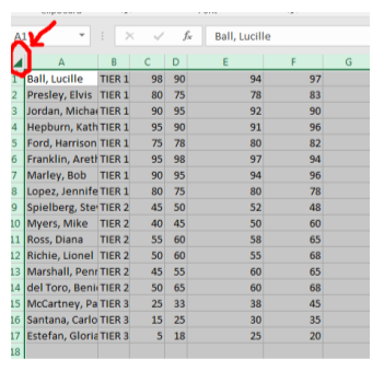
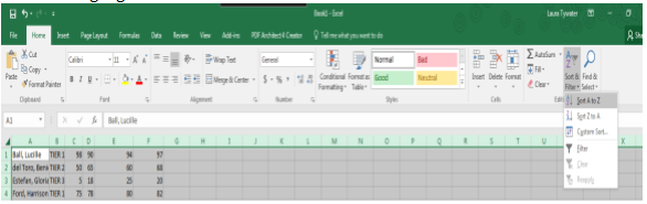
Using the “homeroom” spreadsheet, click the small triangle again in the upper left corner to highlight all of the data and then click “Sort and Filter” and choose “Sort A to Z”
|
|
This will sort the students by the first column in ABC order
Custom Sorting -
|
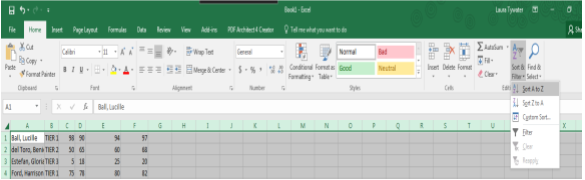
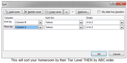
1. Click the small triangle again in the upper left corner to highlight all of the data and then click “Sort and Filter” and choose “Custom Sort”
2. Choose “Add Level” and sort by “Column B” based on values, then by “Column A” based on values. Click ok. |
Through the sort box, you can sort by any column.
A HINT, if you select only one column, it sorts only that column, not the entire document. Make sure you select what you want sorted before or your data will become mixed and confusing.
A HINT, if you select only one column, it sorts only that column, not the entire document. Make sure you select what you want sorted before or your data will become mixed and confusing.
Sort and Filter -
|
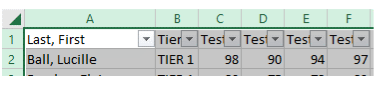
Using the “homeroom” spreadsheet, click the small triangle again in the upper left corner to highlight all of the data and then click “Sort and Filter” and choose “Filter”
|
|
Notice the drop down option for each header. Select Tier and filter by Tier 1. Next, filter by Tier 2.
For Future Reference...Sorting
6. Formatting
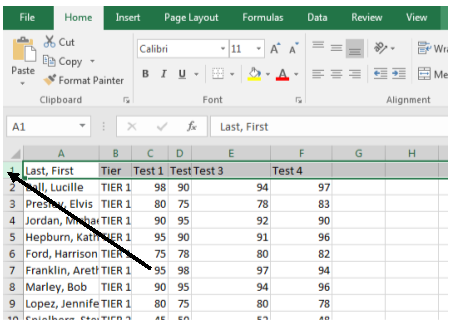
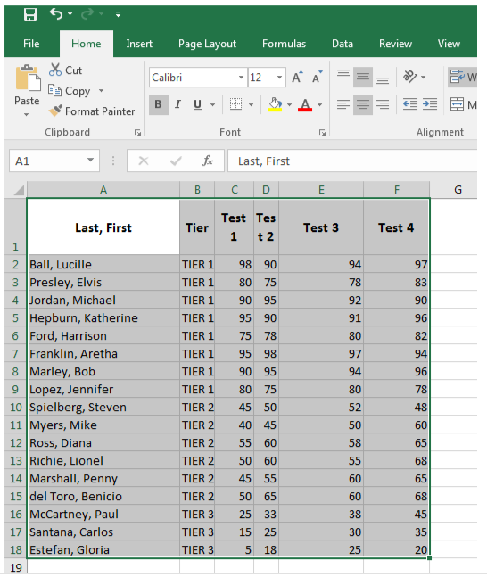
Using the “Homeroom” list which you have opened, click on row 1. The entire row should be highlighted.:
|
1. Using the mouse, place the cursor on this highlighted line and right click with the right mouse button.
2. On the menu that appears, choose Format Cells… 3. Choose the second tab: Alignment. 4. In the box for Horizontal, choose: Center. 5. In the box for Vertical, choose: Center. 6. In the Text control box, click to place a check beside: Wrap text. 7. Then, choose the tab for Font. 8. Choose Font style: Bold Size: 12 and click OK. |
|
9.Choose column A and click the centering button on the Formatting toolbar:
(Everything in the column should center. If it does not, click the centering button one more time. Sometimes it removes the centering command and has to be clicked a second time to apply centering to the entire column.) 10.Center the columns for: Tier, Test 1, Test 2, Test 3, and Test 4 |
|
Borders -
|
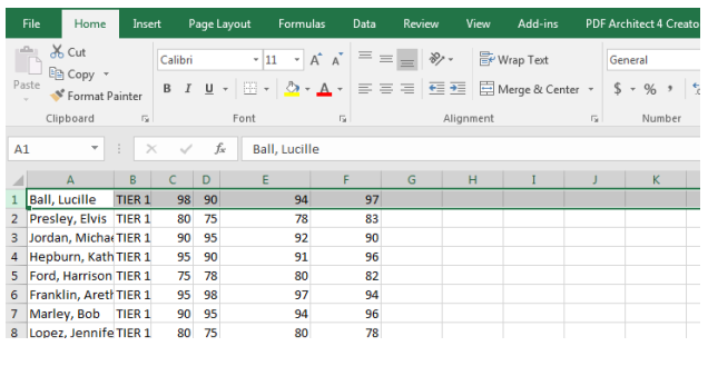
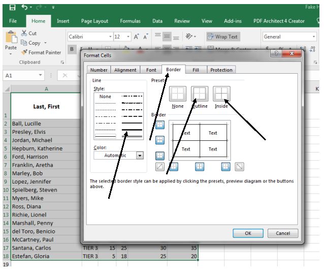
1. Select all cells that have typing in them:
2. Using the mouse, place the cursor on the highlighted area and right click with the right mouse button. On the menu that appears, choose Format Cells… 3. Choose the tab that says Border |
|
4. Under the Style: menu – choose the bold line 5. When the bold line is highlighted, click the button that says: Outline 6. Click the line that shows a narrower line 7. Click the Inside box 8. Click OK 9. Click anywhere on the Excel sheet to turn off the selection of the cells. 10. Your chart should now have a heavy border with thin lines separating all the cells. |
|
Adding Color -
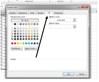

|
1. Select the cells that include the words: Last, First, Tier, Test 1, Test 2, Test 3, and Test 4 2. Right click on the highlighted cells and choose Format Cells again. 3. Choose the tab that says Fill 4. Choose a color. 5. Click OK. 6. Your cells should now be colored. It is possible to type more than one line within one cell. Choose a cell below the last name on the list you just finished formatting. Within the cell, type: This is a test. Hold down the Alt key and press Enter. Type: See it works. Then, press Enter again. Notice that both sentences appear in the same cell. |
For Future Reference...Formatting Cells
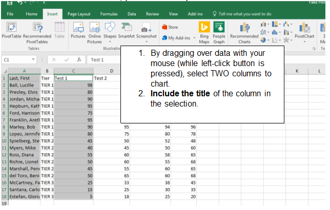
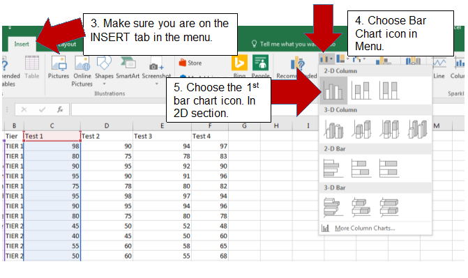
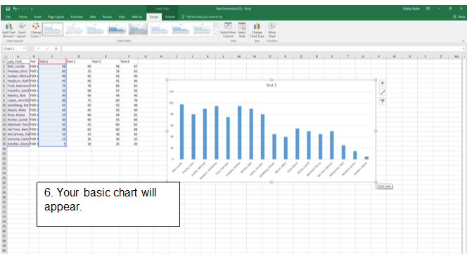
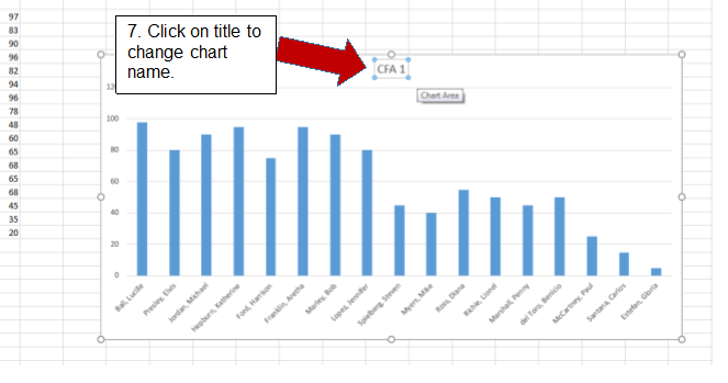
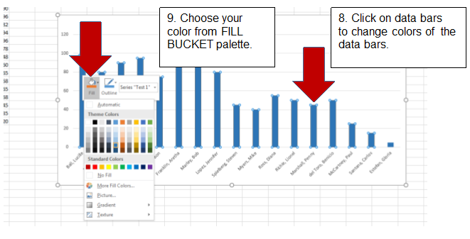
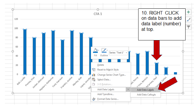
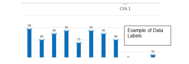
7. Charts and Graphs
For Future Reference...Charts and Graphs